A full proof of Berry-Esseen inequality in the Central Limit Theorem

This proof is based on the book by W. Feller, An Introduction to Probability and its application, volume II and is only for identically independent distributed summands. Thus, I won’t prove the non-identical case because this post will become long. Please find its proof in Feller’s book.

The central limit theorem is concerned with the situation that the limit distribution of the normalized sum is normal as the sample size goes to infinity. But the question you may raise is, “What is the rate of convergence of normalized sum distribution to the standard normal distribution?”. Let’s answer this question by considering the case where the samples are identical. To be more precise, let’s state like this:

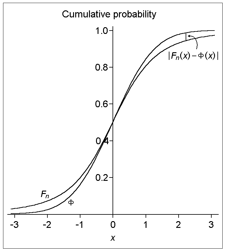
Let $x_{k}$ be independent variable with identical(or common) distribution $F$ such that, $E(x_{k})=0, E(x_{k}^{2})=\sigma^{2}>0,$ $E(|x_{k}|^{3})=\rho<\infty$ and, let $F_{n}$ stands for the distribution of the normalized sum $\frac{x_{1}+x_{2}+\ldots+x_{n}}{\sigma\sqrt{n}}$. Then for all $x$ and $n$, the supremum of convergence between $F_{n}(x)$ and $\phi(x)$ i.e. standard normal distribution is $|F_{n}(x)-\phi(x)|\leq \frac{3\rho}{\sigma^{3}\sqrt{n}}$ .

Looks very boring! Right? Okay, let’s start with the history of the Central limit theorem(CLT).

The first proof of CLT was given by French mathematician Pierre-Simon Laplace in 1810. Fourteen years later, French mathematician Siméon-Denis Poisson improved it and provided us with a more general form of proof. Laplace and his contemporaries were very interested in this theorem because they see the importance of it in repeated measurements of the same quantity. And thus they realized the individual measurements could be viewed as approximately independent and identically distributed, then their mean could be approximated by a normal distribution. Because this statistical plus probability theorem states that for a given sufficiently large sample size from a population with a finite level of variance, the mean of all samples from the same population will be approximately equal to the mean of the population regardless of the shape of the proposed distribution.

Then, the first convergence rate for CLT was estimated by Russian mathematician Aleksandr M. Lyapunov. But, the more refined version of the proof is independently discovered by two mathematicians Andrew C. Berry (in 1941) and Carl-Gustav Esseen (in 1942), who then, continuously refined the convergence theorem of CLT and hence, given this theorem which is named as “Berry-Esseen theorem”. The best thing about this theorem is that it only considered the first three moments.

Now, I think you are very eager to know about the proof of this theorem. Right? Let’s get started without any further delay!

From Feller’s book (Lemma 1 equation 3.13 on page 538), the upper bound between $F_{n}(x)$ and $\phi(x)$ is

$|F_{n}(x)-\phi(x)| \leq \frac{1}{\pi}\int_{-T}^{T}|\frac{\psi(\xi) - \gamma(\xi)}{\xi}| d\xi + \frac{24m}{\pi T}$ $\rule{2cm}{0.4pt}  (1)$

where,

$\psi(\xi)$ = characteristics function for $F_{n}(x)$ which equals to $\psi^{n}(\frac{\xi}{\sigma\sqrt{n}})$,

$\gamma(\xi)$ = characteristics function for $\phi(x)$ which equals to $e^{\frac{-\xi^{2}}{2}}$,

$m$ = maximum growth rate for $\phi$ such that $|\phi^{’}(x)| \leq m < \infty$.

The above expression can be found by starting with Fourier’s methods.  And our proposed proof is based on smoothing inequality (refer Feller’s paper in section 3.5) such that,

$T = \frac{4}{3}\frac{\sigma^{3} \sqrt{n}}{\rho} \leq \frac{4 \sqrt{n}}{3}$.

The last inequality is the result of moment inequality. And, the normal density $\phi$ has maximum $m < \frac{2}{5}$  (I don’t know why Feller chose this bound. I would be very happy if you guys could help me in this quest!).

So equation $(1)$ becomes,

$\pi |F_{n}(x) - \phi(x)| \leq \int_{-T}^{T}|\psi^{n}(\frac{\xi}{\sigma\sqrt{n}}) - e^{\frac{-\xi^{2}}{2}}|\frac{d\xi}{|\xi|} + \frac{24\times 2}{T\times 5}$

$=\int_{-T}^{T}|\psi^{n}(\frac{\xi}{\sigma\sqrt{n}}) - e^{\frac{-\xi^{2}}{2}}|\frac{d\xi}{|\xi|} + \frac{9.6}{T}$ $\rule{2cm}{0.4pt}  (2)$

Now, Let’s find $|\psi^{n}(\frac{\xi}{\sigma\sqrt{n}}) - e^{\frac{-\xi^{2}}{2}}| =$ ?

Isn’t it look like the reverse triangle inequality with exponent “$n$”? I mean this

$|\alpha^{n} - \beta^{n}| \leq n|\alpha - \beta|\Gamma^{n-1}$ if $|\alpha| \leq \Gamma, |\beta| \leq \Gamma$.

Thus, we can say

$|\psi^{n}(\frac{\xi}{\sigma\sqrt{n}}) - (e^{\frac{-\xi^{2}}{2n}})^{n}| \leq n |\psi(\frac{\xi}{\sigma\sqrt{n}}) - e^{\frac{-\xi^{2}}{2n}}|\Gamma^{n-1}$ $\rule{2cm}{0.4pt}  (3)$

, if  $|\psi(\frac{\xi}{\sigma\sqrt{n}})| \leq \Gamma, |e^{\frac{-\xi^{2}}{2n}}| \leq \Gamma$.

Again, let’s make our problem much simpler by proposing $|\psi(\frac{\xi}{\sigma\sqrt{n}}) - e^{\frac{-\xi^{2}}{2n}}| =$?

First of all, let’s suppose $t = \frac{\xi}{\sigma\sqrt{n}}$ so that $\psi(\frac{\xi}{\sigma\sqrt{n}}) = \psi(t)$. Thus, $\xi = t\sigma\sqrt{n}$ so that $e^{\frac{-\xi^{2}}{2n}} = e^{\frac{-t^{2}\sigma^{2}n}{2n}} = e^{\frac{-t^{2}\sigma^{2}}{2}}$.

Look! How beautiful this looks like:

$|\psi(\frac{\xi}{\sigma\sqrt{n}}) - e^{\frac{-\xi^{2}}{2n}}| = |\psi(t) - e^{\frac{-t^{2}\sigma^{2}}{2}}|$

$= |\psi(t) - (1 - \frac{t^{2}\sigma^{2}}{2} + \ldots)|$ , putting the series of $e^{\frac{-t^{2}\sigma^{2}}{2}}$

$= |\psi(t) - 1 + \frac{t^{2}\sigma^{2}}{2}|$ $\rule{2cm}{0.4pt}  (4)$

,  neglecting the higher order terms because for large $n$ then, $t \to 0$.

The characteristics function for $\psi(t)$ is

$\psi(t) = \int_{-\infty}^{\infty} e^{i t x} F_{n}(x) dx$.

From the very first, I said as the sample size goes on increasing the shape of the curve of the proposed distribution tends to match up with the normal curve. I mean this

Isn’t the smoothing concept look like Taylor’s theorem? Exactly! As Taylor’s theorem said we can approximate any curve to a well-defined curve by a series expression. Likewise, we can estimate our proposed distribution with standard normal distribution by taking higher-order terms. So, we will need to go like this

$e^{i t x} = 1 + i t x - \frac{t^{2} x^{2}}{2!} + \sum_{d = 3}^{\infty} \frac{t^{d} x^{d}}{d!}$

or, $\sum_{d = 3}^{\infty} \frac{t^{d} x^{d}}{d!} =e^{i t x} - 1 - i t x + \frac{t^{2} x^{2}}{2!}$.

Now, multiply by $F_{n}(x)$ and do integration both sides with the limit $-\infty$ to $\infty$ i.e.

$\int_{-\infty}^{\infty} (\sum_{d = 3}^{\infty} \frac{t^{d} x^{d}}{d!})F_{n}(x) dx =\int_{-\infty}^{\infty}  (e^{i t x} - 1 - i t x + \frac{t^{2} x^{2}}{2!}) F_{n}(x) dx$ $\rule{2cm}{0.4pt}  (5)$.

From the characteristics property, the subtraction of two characteristics function gives another characteristics function and also we suppose, the result can be approximated by taking the higher order series. This is our trick:

$|\psi(t) - 1 + \frac{t^{2}\sigma^{2}}{2}| \approx |\int_{-\infty}^{\infty} \sum_{d = 3}^{\infty} \frac{t^{d}x^{d}}{d!} F_{n}(x) dx|$

$= |\int_{-\infty}^{\infty} (e^{i t x} - 1 - i t x + \frac{t^{2}x^{2}}{2})F_{n}(x) dx|$ $\rule{2cm}{0.4pt}  (6)$

, from equation $(5)$.

Also, another inequality we can suppose is this:

$(e^{i t x} - 1 - i tx + \frac{t^{2}x^{2}}{2!} + \ldots - \frac{(i t x)^{n-1}}{(n-1)!}) \leq \frac{(x t)^{n}}{n!}$.

For n = 3,

$(e^{i t x} - 1 - i tx + \frac{t^{2}x^{2}}{2!}) \leq \frac{(x t)^{3}}{3!}$.

So, the equation $(6)$ becomes

$|\psi(t) - 1 + \frac{t^{2}\sigma^{2}}{2}| \leq |\int_{-\infty}^{\infty} \frac{(xt)^{3}}{6} F_{n}(x) dx|$.

In the left part of this inequality, we’re going to apply the Cauchy-Schwarz inequality as

$|\psi(t) - 1 + \frac{t^{2}\sigma^{2}}{2}| \leq |\psi(t)| + |\frac{t^{2}\sigma^{2}}{2}|$.

Then, this will turn into

$|\psi(t) - 1 + \frac{t^{2}\sigma^{2}}{2}| \leq|\psi(t)| + |\frac{t^{2}\sigma^{2}}{2}| \leq|\int_{-\infty}^{\infty} \frac{(xt)^{3}}{6} F_{n}(x) dx|$ where the third part of the inequality has a higher value than others.

For our needs, we will use

$|\psi(t)| + |\frac{t^{2}\sigma^{2}}{2}| \leq|\int_{-\infty}^{\infty} \frac{(xt)^{3}}{6} F_{n}(x) dx|$

$\Rightarrow$ $|\psi(t)| + (\frac{t^{2}\sigma^{2}}{2}) \leq \frac{|t|^{3}}{6} |\int_{-\infty}^{\infty} x^{3} F_{n}(x) dx|$, if $\sigma > 0$, and second part is from Cauchy-Schwarz inequality

$\Rightarrow$ $|\psi(t)| + (\frac{t^{2}\sigma^{2}}{2}) \leq \frac{|t|^{3}}{6} \int_{-\infty}^{\infty} |x^{3} F_{n}(x)| dx$, applying the properties of Riemann integral in second part

$\Rightarrow$ $|\psi(t)| + (\frac{t^{2}\sigma^{2}}{2}) \leq \frac{|t|^{3}}{6} \int_{-\infty}^{\infty} |x^{3}| |F_{n}(x)| dx$, applying Cauchy-Schwarz inequality.

$= \frac{|t|^{3}}{6} \times E(|x_{k}|^{3})$

$= \frac{|t|^{3}}{6} \times \rho)$ such that $\rho < \infty$

$\therefore$ $|\psi(t)| \leq 1 - \frac{t^{2}\sigma^{2}}{2} + \frac{1}{6} \rho |t|^{3}$.

Returning back the value of $t = \frac{\xi}{\sigma\sqrt{n}}$. we get,

$|\psi(\frac{\xi}{\sigma\sqrt{n}})| \leq 1 - \frac{\xi^{2}}{2n} + \frac{\rho}{6} \times \frac{|\xi|^{3}}{\sigma^{3} n^{3/2}}$ $\rule{2cm}{0.4pt}  (7)$.

Now, we conclude $|\xi| \leq T$ to smooth our proposed PDF. So that we can use $|\xi| = T = \frac{4}{3}\frac{\sigma^{3}\sqrt{n}}{\rho}$. So, the equation $(7)$ becomes

$|\psi(\frac{\xi}{\sigma\sqrt{n}})| \leq 1 - \frac{\xi^{2}}{2n} + \frac{\rho}{6\sigma^{3}n^{3/2}}|\xi|^{2} |\xi|$

$= 1 - \frac{\xi^{2}}{2n} +\frac{\rho}{6\sigma^{3}n^{3/2}}|\xi|^{2} \times (\frac{4\sigma^{3}\sqrt{n}}{3\rho})$

$= 1- \frac{\xi^{2}}{2n} + \frac{4\xi^{2}}{18n}$

$= 1 - \frac{5\xi^{2}}{18n}$

$\therefore |\psi(\frac{\xi}{\sigma\sqrt{n}})| \leq e^{\frac{-5\xi^2}{18n}}$ $\rule{2cm}{0.4pt}  (8)$

, converting into exponential form with $n \to \infty$.

We know, $\sigma^{3} < \rho$ the assertion of the theorem is trivially true for $\sqrt{n} \leq 3$ and hence we may assume $n\geq 10$.

We take exponent $n-1$ on both sides in equation $(8)$. We can get,

$|\psi(\frac{\xi}{\sigma\sqrt{n}})|^{n-1} \leq e^{\frac{-5\xi^2}{18n}\times (n-1)}$

Thus, for n = 10,

$|\psi(\frac{\xi}{\sigma\sqrt{n}})|^{n-1} \leq e^{\frac{-5\xi^2}{18\times 10}\times (10-1)} = e^{\frac{-\xi^{2}}{4}}$ $\rule{2cm}{0.4pt}  (9)$.

Let me remind you equation $(3)$ with maximum equality i.e.

$|\psi^{n}(\frac{\xi}{\sigma\sqrt{n}}) - (e^{\frac{-\xi^{2}}{2n}})^{n}| = n |\psi(\frac{\xi}{\sigma\sqrt{n}}) - (e^{\frac{-\xi^{2}}{2n}})| \Gamma^{n-1}$ if $|\psi(\frac{\xi}{\sigma\sqrt{n}})| = \Gamma$

So, the right part of equation $(9)$ may serve for the bound $\Gamma^{n-1}$ i.e.

$|\psi(\frac{\xi}{\sigma\sqrt{n}})| = \Gamma$

or, $|\psi(\frac{\xi}{\sigma\sqrt{n}})|^{n-1} = \Gamma^{n-1}$

or, $e^{\frac{-\xi^{2}}{4}} = \Gamma^{n-1}$

Thus, we can have

$|\psi^{n}(\frac{\xi}{\sigma\sqrt{n}}) - (e^{\frac{-\xi^{2}}{2n}})^{n}| = n |\psi(\frac{\xi}{\sigma\sqrt{n}}) - (e^{\frac{-\xi^{2}}{2n}})|e^{\frac{-\xi^{2}}{4}}$ $\rule{2cm}{0.4pt}  (10)$.

Also, we need to formulate one more inequality. Let’s start with this:

$e^{-x} \leq 1 - x + \frac{x^{2}}{2}$ for $x > 0$

$\Rightarrow$ $e^{-x} - 1 + x \leq \frac{x^{2}}{2}$ $\rule{2cm}{0.4pt}  (11)$.

Oh! I almost forgot. We need to construct something very useful. i.e.

$n |\psi(\frac{\xi}{\sigma\sqrt{n}}) - e^{\frac{-\xi^{2}}{2n}}| \leq n|\psi(\frac{\xi}{\sigma\sqrt{n}}) - 1 + \frac{\xi^{2}}{2n}| + n|1 - \frac{\xi^{2}}{2n} - e^{\frac{-\xi^{2}}{2n}}|$, I have added two terms and applied triangle inequality.

$=$ First term $+$ Second term $\rule{2cm}{0.4pt}  (12)$

which means,

First term = $n|\psi(\frac{\xi}{\sigma\sqrt{n}}) - 1 + \frac{\xi^{2}}{2n}| \leq \frac{\rho |\xi|^{3}}{6 \sigma^{3}n^{3/2}}\times n = \frac{\rho |\xi|^{3}}{6 \sigma^{3}n^{1/2}}$, from equation $(7)$.

and,

Second term = $n|1 - \frac{\xi^{2}}{2n} - e^{\frac{-\xi^{2}}{2n}}| \leq n \times \frac{1}{2} \times \frac{\xi^{4}}{(2n)^{2}} = \frac{1}{8n}\xi^{4}$, from equation $(11)$.

Returning the above results in equation $(12)$. we get,

$n |\psi(\frac{\xi}{\sigma\sqrt{n}}) - e^{\frac{-\xi^{2}}{2n}}| \leq\frac{\rho |\xi|^{3}}{6 \sigma^{3}n^{1/2}} +\frac{1}{8n}\xi^{4}$.

Since $\sqrt{n} > 3$, the above inequality should follow the integrand $(2)$ which means

$\pi |F_{n}(x) - \phi(x)| \leq \int_{-T}^{T} |\psi^{n}(\frac{\xi}{\sigma\sqrt{n}}) - (e^{\frac{-\xi^{2}}{2n}})^{n}| \frac{d\xi}{|\xi|} + \frac{9.6}{T}$

$\leq \int_{-T}^{T}n |\psi(\frac{\xi}{\sigma\sqrt{n}}) - (e^{\frac{-\xi^{2}}{2n}})| e^{\frac{-\xi^{2}}{4}} \frac{d\xi}{|\xi|} + \frac{9.6}{T}$, from equation $(10)$

$\leq \int_{-T}^{T} (\frac{\rho |\xi|^{3}}{6 \sigma^{3}n^{1/2}} +\frac{1}{8n}\xi^{4})\times \frac{1}{|\xi|} \times e^{\frac{-\xi^{2}}{4}} d\xi + \frac{9.6}{T}$

$= \int_{-T}^{T} \frac{\rho}{6\sigma^{3}\sqrt{n}} |\xi|^{2} e^{\frac{-\xi^{2}}{4}} d\xi + \int_{-T}^{T} \frac{\xi^{3}}{8n} e^{\frac{-\xi^{2}}{4}} d\xi + \frac{9.6}{T}$ $\rule{2cm}{0.4pt}  (13)$.

Also, we know $T = \frac{4\sigma^{3}\sqrt{n}}{3\rho}$. So,

$\frac{9.6}{T} =\frac{9.6\times 3\rho}{4\sigma^{3}\sqrt{n}} =\frac{36\rho}{5\sigma^{3}\sqrt{n}}$.

From equation (13), let’s consider for $n \to \infty$ then, $T \to \infty$ thus,

$I_{1} = \int_{-\infty}^{\infty} |\xi|^{2} e^{\frac{-\xi^{2}}{4}} d\xi = 4\sqrt{\pi}$

and,

$I_{2} = \int_{-\infty}^{\infty} \xi^{3} e^{\frac{-\xi^{2}}{4}} d\xi = 0$.

These above integrations can be done by using by-parts rule and also from Gamma function. But, I found a difficulty when solving on $\int_{-a}^{a} |\xi|^{2} e^{\frac{-\xi^{2}}{4}} d\xi$. If you guys solve it, please share your solution in the comment box. Thanks in advance!

So, equation $(13)$ becomes

$\pi |F_{n}(x) - \phi(x)| \leq \frac{\rho}{6 \sigma^{3} \sqrt{n}} \times 4\sqrt{\pi} + \frac{36\rho}{5\sigma^{3}\sqrt{n}} = 8.382\times\frac{\rho}{\sigma^{3} \sqrt{n}}$.

$\therefore |F_{n}(x) - \phi(x)| \leq 2.668\times\frac{\rho}{\sigma^{3} \sqrt{n}}$

For simplicity, we use the below as the final form:

$|F_{n}(x) - \phi(x)| \leq \frac{3\rho}{\sigma^{3} \sqrt{n}}$   Q.E.D.